Bayesian Regression - Part 1
09 Dec 2024 - Daniel Sherwood
I will admit that the Bayesian approach to statistical modeling is not perfect. There are some who treat the word Bayesian as a slur, and others who treat it as a sacrament to be enjoyed by the holy few. I am a little more ambivalent. Bayesian modeling requires one to specify prior distributions for the variables one is modeling. I’ve personally found it difficult to justify why one distribution should be used as my prior versus another. But I am getting ahead of myself. I have three separate posts in mind to explain my thoughts. The first, this post, will be about how similar Bayesian and orinary regression are to each other. The second will go into more details as to how they differ, and the third will talk about implications for prediction.
As a refresher, here is the maximum likelihood formulation used in Frequentist/ordinary regression:
$\log L(\beta | X, y) = -\frac{n}{2}\log(2\pi\sigma^2) - \frac{1}{2\sigma^2} \sum_{i=1}^{n} (y_i - x_i^T\beta)^2$
And here is the mathematical formulation for Bayesian regression:
$p(\beta | X, y, \sigma^2) = \frac{p(y | X, \beta, \sigma^2) \cdot p(\beta)}{\int p(y | X, \beta, \sigma^2) \cdot p(\beta) d\beta}$
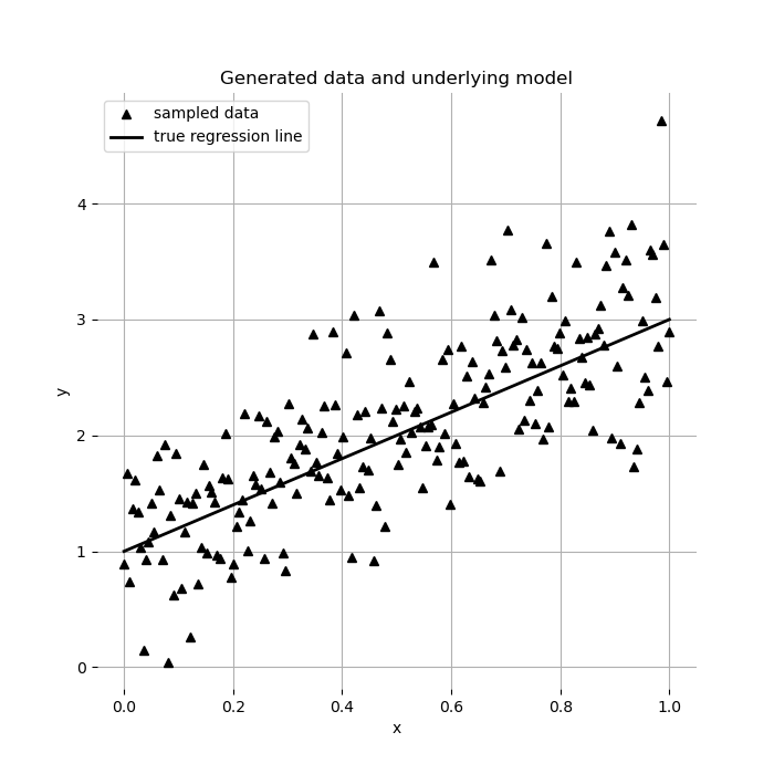
1. Generate Some Data
The first thing we will do is generate some data. The following piece of code is copied straight from a PYMC notebook.
import numpy as np

size = 200
true_intercept = 1
true_slope = 2

x = np.linspace(0, 1, size)
# y = a + b*x
true_regression_line = true_intercept + true_slope * x
# add noise
y = true_regression_line + rng.normal(scale=0.5, size=size)
here’s the data we generated. The code for the figure is also from the same notebook, but altered slightly to match the theme of this blog post.
2. Recover Parameters with Statsmodels
Let’s use the statsmodel python package to recover the parameters. This is fairly straightforward.
import statsmodels.api as sm
x = sm.add_constant(x)
model = sm.OLS(y,x)
results = model.fit()
print(results.params)
the results of which are as follows:
| Mean | LwrConf | UprConf | |
|---|---|---|---|
| Slope | 2.06 | 1.809 | 2.310 |
| Intercept | 1.05 | 0.901 | 1.191 |
3. Recover Parameters with PYMC
Now let’s perform a basic regression with PYMC. This is a little more involved, making use of a python context via
with.
from pymc import Model, Normal, sample, Uniform
with Model() as model:

    sigma = Uniform("sigma", -10, 10)
    intercept = Uniform("intercept", -10, 10)
    slope = Uniform("slope", -10, 10)

    likelihood = Normal("y", mu=intercept + slope * x, sigma=sigma, observed=y)

    idata = sample(3000)

print(az.summary(idata, var_names=["intercept","slope"], hdi_prob=0.95, fmt='long'))
the results are very close!
| Mean | LwrConf | UprConf | |
|---|---|---|---|
| Slope | 2.06 | 1.815 | 2.306 |
| Intercept | 1.05 | 0.904 | 1.190 |
4. Discussion
In the first example, the OLS model used maximum likelihood to determine the slope and intercept. Tests were perfomed, and the relevant statistic was used to create a confidence interval around the parameter. A 95% confidence interval states that 95 out of 100 similar intervals will contain the parameter. This has been causing confusion for decades. The results from Bayesian Linear Regression, however, mean something a bit different. What is essentially happening is that a multitude of slopes and intercepts have been calculated, resulting in a distribution of our parameters. A credible interval surrounding our parameter states that 95 out of 100 slopes parameters will be within the interval. This makes much more intuitive sense.
You can see that Bayesian Linear Regression almost exactly equals Frequentist Linear regression when the prior distribution specified for the parameters is uniform. We assumed absolutely no knowledge about our slope or intercept and our Bayesian results matched our OlS results. So, in a way, you can think of frequentist approaches as doing the same: they assume nothing about the data. This philosophy is the primary point of contention between Bayesian-ists and Frequentists. Should you assume things about your data or not? That’s the question.